

In his foundational 2014 research, Michael Kitces rightly dismantled the myth of the psychological bucket strategy, proving that arbitrary time segmentation with basic decision rules amounts to little more than a behavioral illusion. We completely agree: unscientific bucketing fails the math of long-term wealth preservation.
However, the psychological appeal of bucketing wasn’t the problem, the lack of structural engineering was. Traditional “buckets” are simply Total Return in disguise. By using a formal Asset-Liability Matching (ALM) framework, we can anchor cash flows to true structural horizons, marrying Kitces’ total-return discipline with institutional-style liability-driven investing (LDI).
Executive Summary
Bucketing strategies are popular with financial advisors and retail investors because they are easily understandable and mesh well with the financial planning process as they apply an intuitive, somewhat temporal investment solution. In this piece, we will show why traditional bucketing strategies are imperfect at best, and how an institutional-style ALM strategy improves both financial planning and investment management, resulting in an overall methodology that enhances, rather than replaces, traditional Total Return processes.
S1 – Buckets, LDI & ALM: Cutting Through the Confusion
It is useful to outline exactly what we are discussing because while all ALM/LDI strategies utilize time-segmented pools, all bucketing strategies are not ALM.
There are generally two ways to construct portfolios:
- The Total Return (TR) Approach: Starts with the asset side of the balance sheet. It focuses on optimizing a single pool of capital for maximum risk-adjusted efficiency relative to a market benchmark (such as the S&P 500 or a 60/40 index). TR assumes the client can tolerate the volatility of the entire pool so long as the long-term average return is sufficient.
- The Asset-Liability Matching (ALM) Process: Starts with the liability side of the ledger. It quantifies the exact time horizons over which cash will be needed. For a household, any future goal requiring cash is a liability that must be mapped to an asset of corresponding future expected real value.
Under ALM, wealth is managed not as a single homogeneous pool, but as a series of interrelated strategies engineered to serve distinct temporal needs. Risk is not defined by price volatility or tracking error; it is measured by whether the investor can fund future cash obligations with reliability. The benchmark shifts from “Did we beat the market?” to “Did we have the money when we needed it?”
Buckets were originally popularized by Harold Evensky in 1985 as the Cash Flow Reserve strategy. While framed as a bucket strategy, it was actually a TR strategy disguised as a bucket to solve a purely psychological friction. Evensky’s model included a small cash reserve (1–2 years of expenses) with the remaining 90%+ of the portfolio allocated to a traditional MPT framework.
Kitces (2014) correctly dismantled the math of these generalized, vague bucket systems. However, the evolution of wealth management requires us to move past both behavioral illusions and the sequence-of-returns vulnerability of pure Total Return. By replacing arbitrary mental accounting with rigorous ALM, we transform the bucket from a psychological gimmick into a mathematically sound immunization tool.
S2 – Retirees are Pension Funds.
A retiree with a 30-year horizon faces a stream of nominal and real liability obligations across a known time structure. This is precisely the problem pension funds and insurance general accounts have solved through LDI for decades. The retail planning industry is an outlier, pretending that households should be managed on single-allocation, pool-based principles that institutional giants discarded long ago.
While some advisors argue that retail investors lack predictable cash flows, we find the opposite. Retail investors have highly identifiable structural events: monthly living expenses, weddings, college funding, auto purchases, healthcare transitions and multi-generational needs. They do not think in singular, homogeneous time horizons. They think in temporal goals: “Can I buy a house in 2 years? Can I send my child to college in 15 years? Can I retire in 20?”
More importantly, the retail investor, unconstrained by strict institutional mandates or regulatory straightjackets, has a nearly unimpeded menu of asset options to implement ALM effectively.
S3 – The Equity Problem: Quantifying “The Long Run”
When I worked with banks on ALM strategies during the financial crisis, I was consistently frustrated by their inability to utilize equity allocations or multi-asset instruments in their ALM methodologies. Although equities will outperform bonds in 95% of rolling 20-year outcomes, many banks matching 20-year time horizons are constrained only to high-quality fixed income assets. This is because the equity market is more akin to a perpetual instrument than a fixed temporal instrument like a 20-year bond. And while a 20-year equity horizon has a high probability of positive real returns, it does not have a 100% chance of positive real returns. The phrase “stocks for the long run” is a hope, not a horizon. For a rigorous ALM application, hope is not a risk-management input; you must quantify the timeline required for the equity market to clear its sequence risk.
Corey Hoffstein makes an important distinction in thinking about ALM across time horizons: there is explicit ALM and statistical ALM. When you match a 6-month T-Bill of $50,000 to a $50,000 car purchase in 7 months, you’re making an explicit ALM allocation—the match is mechanical and certain. When you match $100,000 of today’s S&P 500 to a 20-year retirement goal, you’re making a statistical ALM allocation where the realized outcome will land somewhere along a wider distribution.
The Defined Duration methodology is an ALM strategy that seeks to close and clarify this statistical and explicit gap by looking at the equity market as a stream of future real cash flows with a certain amount of sequence risk we can quantify. We define the Defined Duration (DD) as the compound time horizon required to achieve a real terms breakeven following a maximum drawdown:
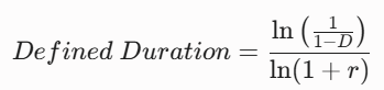
Where:
- D = The maximum anticipated real drawdown risk (e.g., 50%)
- r = The expected real return based on current valuations (e.g., a CAPE ratio of 30 implies a 1/30 or 3.33% real return)
Under these conditions, a portfolio dropping 50% requires a 100% real return to break even. Compounding at a 3.33% expected real return, the math yields a Defined Duration of 21.16 years:

NB – One might assume this is being overly conservative as the expected return might increase when markets decline, however, our baseline assumption to reduce sequence risk is to plan for the worst and hope for the best.
Now that the equity time horizon is quantified, the investor can actually apply a matching process that goes beyond simple fixed income matching processes like bond ladders. In fact, they can blend instruments that enhance and bridge the gap between equities and bonds so we can enhance ALM processes in more complete “asset laddering” approaches. For instance, we can utilize a 60/40 stock/bond instrument in an ALM process by quantifying the Defined Duration of the stock and bond markets and then using the instrument as a blended duration instrument that matches to, for example, 12 year time horizons and helps mitigate sequence risk while also enhancing returns relative to a similar 12 year bond instrument. Total Return instruments need not be adversaries of ALM – they can be inputs that enhance the entire methodology.
Case Study: The Asset Ladder in Practice
Let’s take a household with the following profile:
- Profile: Two 55-year-old spouses, earning $150,000 after-tax income, $125,000 annual expenses, and $2,000,000 of liquid investable assets.
- Goals & Liabilities:
- New $60,000 car in 6 months.
- $75K for daughter’s wedding in 2 years.
- $50K for new bathroom remodel in year 3.
- $100K house down payment for retirement downsizing in year 7 in preparation for retirement downshift.
- Comfortably fund ongoing retirement spending needs.
This set of expenses can be applied to a customized set of assets. For instance, you could map out a staggered bond ladder of TIPS and/or T-Bills to match the known 0-7-year expenses precisely. In other words, this could be done in a highly granular fashion where specific goals are pinned to inflation-adjusted assets of the correct corresponding quantity. When near-term liabilities are correctly quantified, there is no need for strict rebalancing rules or some vague set of decision trees because the financial needs of the investor dictate whether rebalancing is needed in the short term.
To match the household’s exact $2,000,000 balance, the structured asset ladder is detailed below (this example is simplified for illustrative purposes):
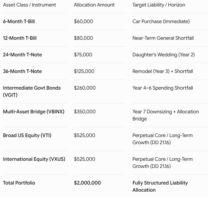
This allocation sits at roughly 63/37 stocks/bonds in aggregate. But unlike a simple 60/40 portfolio (such as VBINX), which serves a single long-term time horizon, the instruments are disaggregated. Despite having a similar risk/return profile to a 60/40 pool in aggregate, the investor has virtually eliminated sequence risk relative to their near-term goals. Each asset is cleanly mapped to a specific goal with an inflation-adjusted buffer. The bond ladder serves as a rolling certainty element, while our longer-term instruments are constant maturity bond or cap-weighted equity instruments.
Although longer-term retirement planning goals are more unpredictable, the process matches equities to longer duration instruments to help the investor take advantage of the temporal flexibility they have there. Additionally, multi-asset instruments like VBINX still serve a purpose in the portfolio as they help bridge the gap between our long and short duration instruments to help smooth returns and provide optionality in the portfolio should we need to rebalance in the future.
This portfolio isn’t just a blob of diversified assets targeting a Total Return strategy. It is a structured set of assets matched to specific personalized planning goals. This portfolio communicates real goals and purpose to the investor, while the 60/40 Total Return portfolio communicates little more than hopeful returns with unknown sequence risk. If you’ve ever had to tell an investor to “stay the course” using some iteration of Total Return 60/40, then this temporal uncertainty is precisely the cause. A structured ALM process eliminates that problem because the portfolio’s different elements have clearly defined goals.
S4 – Why ALM Processes Are Superior
1. ALM Processes Are Inherently Planning-Based
An ALM process necessarily starts with the liability side of the balance sheet and matches the assets to correspond. This process must begin with rigorous financial planning and personal conversations that establish a clear connection between the advisor, the client, and their goals in working together. This isn’t a vague risk profiling process or age-based investment management process. It is a personal discussion about what matters to a person and the specific goals and needs they have over their life. This includes personal expenditures, child planning, succession planning, and multi-generational needs. These aren’t just numbers in a Total Return projection, they are the things that will help us make our lives more predictable and our goals more attainable.
Perhaps more importantly, because the process is planning-based, the benchmark changes. A Total Return process is a performance competition, which creates behavioral and portfolio management conflicts. When the benchmark is a long-term instrument (like the S&P 500) measured against an annual goal (like annual reviews), the client is consistently under the impression that the portfolio is in a risk-adjusted return competition with everyone else. The benchmark should be a temporal benchmark based on whether you are able to fund your needs. The Total Return process establishes unrealistic expectations upfront, expectations that the advisor will inevitably have to apologize for not meeting at times.
2. ALM Processes Are More Understandable
It is not uncommon to hear that bucketing style strategies are little more than “mental accounting.” I don’t view ALM processes as mental accounting so much as I view them as sound financial planning. Total Return strategies don’t give the investor an understanding of the time horizons over which they can fund their spending goals. In this sense, their main weakness is that the spending is not mentally accounted for. Mental accounting, or quantifying the future accounting needs of the portfolio, is not a weakness, it is the strategy’s primary strength, assuming the accounting and planning is done rigorously.
Human beings do not navigate the financial world thinking in terms of alphas, betas, style boxes and factors. They navigate the financial world as a sequence of events across time. They want to know when they can retire and how they can pay for things at certain times. ALM processes provide clarity to these questions and are therefore intuitive to the end investor. When you can tell someone that they have a precise amount of months blocked out for monthly withdrawals, house down payments, and other goals, you are giving them clarity through proper accounting. You are now communicating everything through a language (time) that is universal, instead of the current factor and style-based jargon that only compounds confusion in Total Return strategies.
3. Decision Rules Do Not Dictate the Portfolio’s Changes; Optionality and Structural Temporal Diversification Do
ALM strategies are specifically diversified across the entire liability curve. This process should create what essentially looks like an enhanced asset ladder where the assets are laddered out over the entire curve in sequence. Kitces (2014) correctly identifies the flaw in the decision tree utilized by some bucketing strategies. But the very first decision rule breaks the most essential rules of ALM:
“1) If equities are up, take the retirement spending from equities”
Treating a 21-year statistical asset as a 1-year funding source simply because its price went up isn’t dynamic rebalancing in an ALM framework; it is a violation of the portfolio’s structural design. The investor with a 10-rung, 10-year bond ladder does not fund year 1 liabilities from the 10th rung simply because 10-year bond prices go up in year 1. That is counter to the very structure of the ladder. They are using a 10-year bond specifically because they expect it to generate a superior return by year 10. Treating the long-duration instrument as a 1-year funding instrument is no different than the Total Return strategy that tries to turn a 60/40 mix into an annual funding instrument. This is antithetical to the entire purpose of ALM.
Like a multi-rung bond ladder, a rigorous ALM portfolio should follow a time-weighted process where time horizons and needs dictate portfolio changes. When the 1-year T-Bill matures, the balance is liquidated or reinvested into a longer-term asset. There is no complex decision tree in this process. Time and needs dictate the size of rebalancing. And if the investor is allocated properly across the curve, they should have a reasonably high expectation of being able to fund and rebalance from the longer duration instruments across time. This asset laddering structure with its specific temporal allocations is what dictates future portfolio changes.
In our previous example, the portfolio still has significant duration skew before rebalancing is required, as our near-term assets are perfectly matched out to year 3. Theoretically, the ladder could be extended further, but even in this simple example, we experience three years of duration insulation before any rebalancing is required to refill our short-term bucket. Temporal diversification isn’t just an asset class diversifier; it is a structure that gives the investor optionality and the ability to wait patiently for longer-term instruments to accrue the returns we require from them.
A common critique of bucketing strategies is “but how do you refill the short-term bucket.” This problem isn’t unique to bucketing and ALM strategies. It is a problem for ANY portfolio that involves a withdrawal requirement. The difference between the Total Return and the ALM strategy is your ALM portfolio should give you enhanced funding optionality if it’s allocated over numerous distinct time horizons.
4. Potential for Superior Returns due to Duration Drift and Risk Capacity
ALM strategies should often start and recalibrate to higher expected returns due to the mechanical nature of their structure and process. Imprecise and subjective financial planning often results in holding far more bonds than an investor actually requires. For instance, traditional rules like the “age in bonds” rule or “age minus 10%” will result in structurally bond-heavy portfolios later in life. Kitces and Pfau (2014) found that a rising equity glidepath can often better serve an investor. This is precisely what a well-structured ALM portfolio should achieve.
By starting the process with a needs-based fixed income allocation, the planner allocates to bonds strictly with what is needed. If we rigorously quantify liabilities out to 7 years, then we can build a needs-based fixed income allocation and match the remainder of the assets to longer-term multi-asset instruments and equities. This provides the best of all worlds where the investor has a front-loaded set of certainty with long-term growth assets matched to corresponding long-term growth needs. This needs-based approach establishes a quantified bond bucket that will often generate a superior starting expected return when compared to more traditional TR rules.
As an example, if a retired 70-year-old investor has a $50K annual shortfall versus Social Security with a $2MM portfolio, they have a vastly different risk capacity compared to an investor with a $10MM portfolio and the same $50K annual shortfall. Investor B has a higher risk capacity because they manage their liabilities better on a relative basis. This frees up capacity to take more temporal risk because they do not need to fund the same relative balance in the near term. While a Total Return approach might say both of these investors should follow something close to an age minus 10% rule, the ALM process comes to a totally different conclusion and says these investors are fundamentally different because their financial risk capacity is different. Behavior should not drive asset allocation. Risk capacity based on financial health should drive asset allocation. Working from the liability side of the balance sheet is the optimal way to quantify one’s risk capacity.
Perhaps most importantly, the very structure of the ALM portfolio should help generate superior returns relative to the same starting Total Return portfolio due to duration skew embedded in the funding mechanism. If an investor starts with a static 63/37 portfolio (such as 63% in VT and 37% in BNDW) versus our aforementioned structured portfolio, the ALM portfolio incurs an inherent duration drift. There is no decision tree requiring an annual reset to the 63/37 because the portfolio isn’t required to reset every year. You certainly aren’t reducing your long-duration equity component just because “equities are up.” You are intentionally allowing your long duration instruments to grow while you fund your short-term goals from mechanically matched instruments. As you consume the short-term instruments you are allowing your overall portfolio duration (and expected returns) to increase instead of mechanically rebalancing back to 63/37 every year.
Meanwhile, the investor with a systematic TR strategy will rebalance every year to the same general temporal profile. The ALM investor, on the other hand, is letting their average temporal target drift as they draw down short-term instruments. This causes a mechanical increase in the average time horizon of the overall portfolio that only resets when you choose to reset it. This means we are doing exactly what Kitces and Pfau advocate in the rising glidepath rule. As we spend down the near-term assets, the portfolio’s average time horizon is drifting ever longer until we choose to reset it. Letting the duration of the aggregate portfolio drift over time is a feature of ALM, not a bug.
Lastly, this process creates clarity and aligns assets to proper time horizons. If equities are matched to a 21-year target, they are not to be judged on a 21-month time horizon because the ALM portfolio has shorter-duration instruments covering that period of concern. This compartmentalization of assets creates behavioral bandwidth that allows the investor to behave better because they can understand the exact purpose of their assets within the portfolio.
Conclusion
I am wholly convinced that ALM methodologies will be the dominant way in which retail financial planning and investment management will be done in the future. And while this process is well understood in the institutional investment management world, it is largely undiscovered in the retail investment management world. If you are an advisor utilizing ALM processes and you would like to collaborate with us, please reach out to me here.